Probabilistic Forecasting

In Part 1 of this series we discussed how probabilistic forecasting retains each estimate’s uncertainty throughout the forecast. We looked at how weather forecaster’s present uncertainty in their predictions and how people seem comfortable that the future cannot be predicted perfectly and life still continues. We need this realization in IT forecasts!

In Part 2 we look at the approach taken in the field of probabilistic forecasting, continuing our weather prediction analogy.

We can observe the present with certainty. Meteorologists have been recording various input measure for years, and evidence suggests ancient cultures have understood the seasons to the extent they knew what food items to plant and when. These observations and how they played out over time form the basis for tomorrow’s weather forecast. Modern forecasters combine today’s actual weather conditions with historical observations and trends, using computer models.

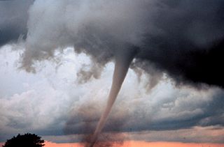
With many historical observations for each measure (temperature range for the same day over the past thirty years for example), we can see patterns. Probabilistic forecasting incorporates the observed pattern rather than just one individual measure. This retains valuable uncertainty information, maintaining a full range of possibilities rather then emphasizing one. Collections of multiple measures are called a “Probability Distributions.” A Probability Distribution represents how frequently different values occur. Emphasis on frequency helps predict which outcomes are more likely than others. For example, although a tornado is possible (occurred once before in the last 100 years,) we will only close schools if the likelihood of a tornado exceeds a threshold of risk, for example, 5%. To do otherwise would be economically and socially unacceptable. We live in an uncertain world and we empower our weather forecasters and leaders to make informed judgments. They sometimes get it wrong. Though popular news might have you think otherwise, we usually understand when decisions based probabilistic forecasts are wrong.

Combining uncertain inputs (creating joint probability distributions) is the trick to responsible forecasting. Mainstream weather forecasters model weather by simulating many possible outcomes using historical data and computing the likelihood of any possible outcome.

For example, if there are two corners with unsynchronized traffic lights on your drive to work, there are four possible combinations of impact to your commute. Both sets are green, you hit one of the lights but not the other (two combinations), or you hit both sets of lights. Your chance of hitting 2 green lights is 1 in 4.

When the weather forecaster says 75% chance of rain, they most often^ mean that 75% of their model results showed rain in your area. They have simulated thousands (or hundreds of thousands) of weather outcomes and counted the number that forecast rain versus the total: this is the probability of rain. Each simulation uses different input starting values chosen randomly from historic observations, and then simulates how these inputs interact and compound in the complex weather system.

^ Sometimes they mean 100% chance of rain in 75% of the area, but this is almost never the case.

Good forecasts require computation time. If there are many input variables, the number of simulations required to get a good result explodes, which explains why forecasters use large computers to forecast climate change and major storms. Also, most good meteorologists run multiple models. Some are good at picking temperature range, and some are good at picking precipitation.

Forecasting is the art of predicting to the best of your ability, seeing if it comes to fruition, and learning from that. How do forecasters know which model to trust? They find out tomorrow which one is right, and favor that model in the future! This feedback loop improves the models over time, which explains why forecasts are rarely completely wrong unless there is severe weather operating at the boundary of modeling behavior.

The process we just described is called “Monte Carlo simulation”. It is the “addition operator for uncertainty”. It is the main tool used for understanding risk and outcomes in fields like mineral exploration, insurance, and finance (nobody said the models are perfect yet!).

IT project forecasting carries a lot of uncertainty. When we estimate or forecast a project or required team size, we should acknowledge and incorporate our uncertainties into our forecasts. Commonly available tools fail to do this. We look stunned every time these estimates turn out wrong, but given the naive approaches we use, it should be no surprise.

In the next part of this series we will examine what to do when historical data isn’t available. Future parts of this series will examine specifically at how IT forecasting uncertainty can be predicted and improved.